
Numerical Integration/Differentiation in R: FTIR Spectra
Posted: Tuesday, February 23rd, 2010
Stumbled upon an excellent example of how to perform numerical integration in R. Below is an example of piece-wise linear and spline fits to FTIR data, and the resulting computed area under the curve. With a high density of points, it seems like the linear approximation is most efficient and sufficiently accurate. With very large sequences, it may be necessary to adjust the value passed to the subdivisions argument of integrate(). Strangely, larger values seem to solve problems encountered with large datasets...
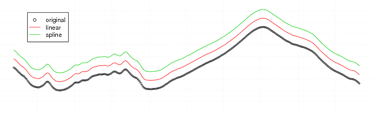
FIgure: FTIR Spectra Integration
Implementation
# numerical integration in R
# example based on: http://tolstoy.newcastle.edu.au/R/help/04/10/6138.html

# sample data: FTIR spectra
x <- read.csv(url('http://casoilresource.lawr.ucdavis.edu/drupal/files/fresh_li_material.CSV'), header=FALSE)[100:400,]
names(x) <- c('wavenumber','intensity')

# fit a piece-wise linear function
fx.linear <- approxfun(x$wavenumber, x$intensity)

# integrate this function, over the original limits of x
Fx.linear <- integrate(fx.linear, min(x$wavenumber), max(x$wavenumber))

# fit a smooth spline, and return a function describing it
fx.spline <- splinefun(x$wavenumber, x$intensity)

# integrate this function, over the original limits of x
Fx.spline <- integrate(fx.spline, min(x$wavenumber), max(x$wavenumber))

# visual check, linear and spline fits shifted up for clarity
par(mar=c(0,0,0,0))
plot(x, type = "p", las=1, axes=FALSE, cex=0.5, ylim=c(0,0.12))
lines(x$wavenumber, fx.linear(x$wavenumber) + 0.01, col=2)
lines(x$wavenumber, fx.spline(x$wavenumber) + 0.02, col=3)
grid(nx=10, col=grey(0.5))
legend(x=615, y=0.11, legend=c('original','linear','spline'), col=1:3, pch=c(1,NA,NA), lty=c(NA, 1, 1), bg='white')

# results are pretty close
data.frame(method=c('linear', 'spline'), area=c(Fx.linear$value, Fx.spline$value), error=c(Fx.linear$abs.error,Fx.spline$abs.error))

  method     area        error
1 linear 27.71536 0.0005727738
2 spline 27.71527 0.0030796529
splinefun() can also compute derivatives
par(mar=c(0,0,0,0), mfcol=c(2,1))
plot(x, type = "l", lwd=2, axes=FALSE)
grid(nx=10, col=grey(0.5))
plot(x$wavenumber, fx.spline(x$wavenumber, deriv=1), type='l', axes=FALSE)
lines(x$wavenumber, fx.spline(x$wavenumber, deriv=2), col='red')
grid(nx=10, col=grey(0.5))
abline(h=0, lty=2)
legend('topright', legend=c('1st derivative','2nd derivative'), lty=1, col=1:2, bg='white')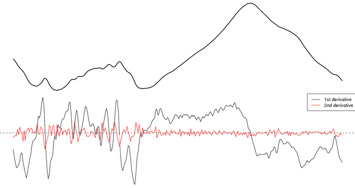
Figure: Numerical Estimation of Derivatives
Attachment:
Links:
Additional Example Using Lattice Graphics
R: advanced statistical package
Plotting XRD (X-Ray Diffraction) Data
