Blog

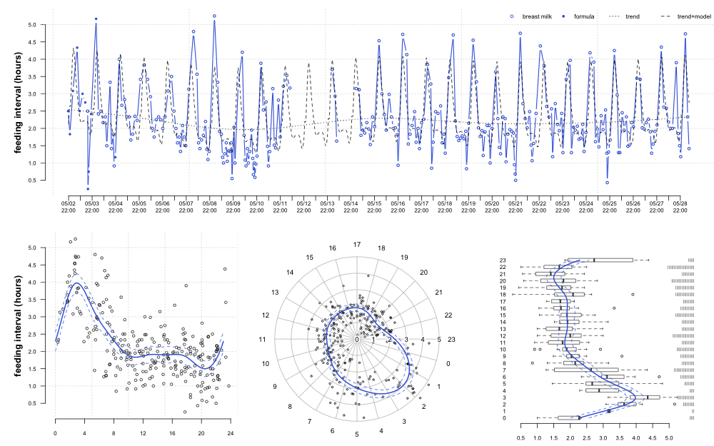
While on paternity leave I had an opportunity to test out periodic smoothing splines (within the framework of generalized additive models) on an interesting time-series-- an infant's feeding schedule.

load / format data and fit GAMs

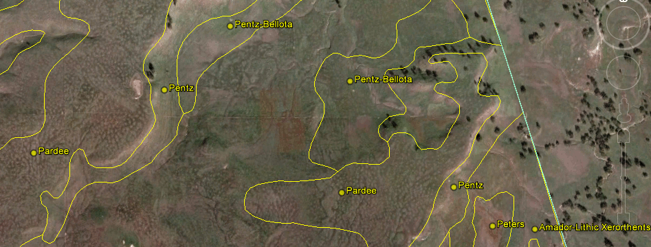
Soil survey data are typically built upon a foundation of soil-landscape relationships that have been verified in the field. SSURGO data contain several geomorphic descriptions of landscape, landform, hillslope position, and surface shape for each soil component. In an ideal setting, suites of soils predictably occur along the standard hillslope positions (summit, shoulder, backslope, footslope, toeslope), forming what is known as a catena. Reality is usually much more complex, and soil component Alpha may actually have been found at several hillslope positions. With a little aggregation and re-formatting of the raw data, it is possible to use SSURGO to produce a probability matrix for a set of named components (e.g. soil series) describing where these soils are most likely to occur. A new function in the sharpshootR package makes this operation very simple.

The CDEC website provides access to a wide range in hydrologic data (stream flow, snow survey, etc.) collected in California. The following code and functions (attached at the bottom of the page) illustrate how to query CDEC, and graphically compare the May 2011 snow survey data with the historic record at 15 sites. Data in this format lend well to the "split-apply-combine" strategy. Integration of several figures (scatter plot, custom box-whisker plot) and graphical legend for bwplot is accomplished via the latticeExtra package. See in-line comments below for a more complete description of the code.

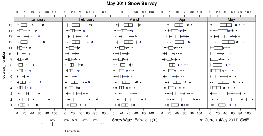
Note that snow water equivalent (SWE) from May 2011 (blue dots) is compared with the historic record (box-whisker plots) for the months of Jan-May. Pretty impressive snowfall!  

Define Custom Functions

Several new AQP-related tutorials have been posted to the R-Forge project page.

1. SoilProfileCollection class/method documentation
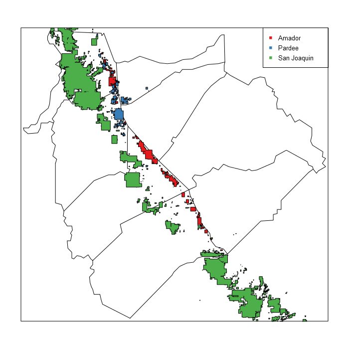
2. soil series extent mapping examples

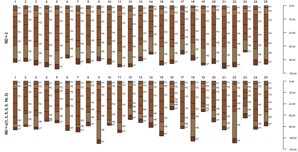
Something fun to play with before the new year: experimental code in aqp for simulating soil profile data from a single "template" profile. The basic idea: simulate horizon thickness data using a family of Gaussian functions with mean defined by horizon thickness values found in the template and standard deviation defined by the user. Larger hz.sd values will yield more drastic variation in the simulated results. Note that only "horizonation" (e.g. the sequence of horizons and their respective thickness) is simulated; horizon attributes (e.g. texture, pH, etc.) are copied from the "template" profile.

Basic usage is demonstrated below, see package manual page for details. This function is only available in the version of aqp hosted by R-Forge. It should be on CRAN by the new year.

UPDATED 2013-04-08

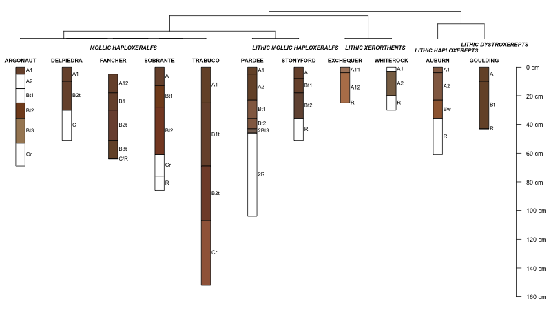
This functionality it now available in the soilDB and sharpshootR packages. All code on this page is now superseded by the fetchOSD() and SoilTaxonomyDendrogram()functions.

UPDATED 2012-11-07

I have been thinking about a URL-based interface to basic Official Soil Series Description (OSD) data for a while now... something that when fed a URL, would return CSV-formatted records to the calling process. These type of interfaces can later be used to support more complicated systems, such as our smartphone interface to SoilWeb. URLs can be accessed like files in R, making it possible to do something like this:

OSD Site-Level Data

R provides several frameworks for composing figures. Base graphics is the simplest, grid is more advanced, and the lattice/ggplot packages provide convenient abstractions of the grid graphics system. Multi-element figures can be readily created in base graphics using either par() or layout(), with analogous functions available in grid. Mixing the two systems is a little more complicated, somewhat fragile, but entirely possible.

I recently needed to combine base+grid graphics on a single page; two sets of base graphics on the left, and the output from xyplot() (grid) on the right. Following some tips from Paul Murrell posted on r-help, the solution was fairly simple. A truncated example of the processes is listed below, corresponding to the attached figure. While the result was "good enough" for a quick summary, there are clearly some improvements that would make figure more useful.

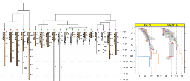
Image: Mehrten Soil Summary