
Islands of Fertility: Oak Tree vs. Buckwheat Savannah Soils
Between Sandy Creek and Chalone Creek, waypoints ending in -P006 through -P009.
Samples collected under Live Oak (SSGG-spring-05-P006, SSGG-spring-05-P009) correspond to the soil described at pit S04CA069007K (Corralitos). Samples collected under Buckwheat (SSGG-spring-05-P007, SSGG-spring-05-P008) correspond to the soil described at pit S04CA069004K (Toags). Bulk density data were collected via ring method at all 4 locations. Compliant-cavity method data were taken at pits P006 and P007.
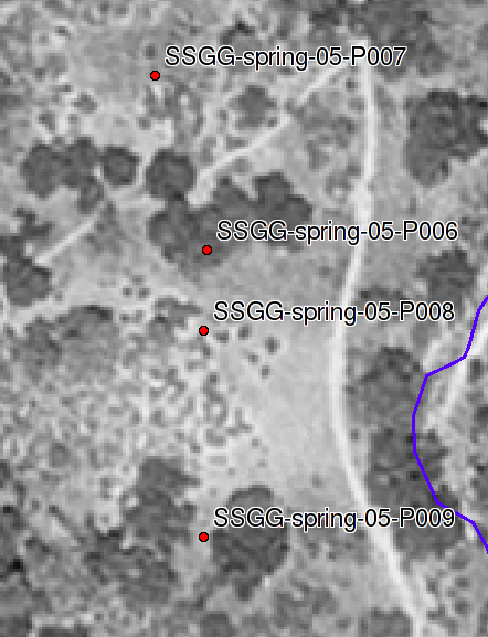
Islands of Fertility: Sample Sites: Sample sites for islands of fertility project. Pits were described and sampled by the Soils and Biogeochemistry Graduate Group, Feb. 2005.
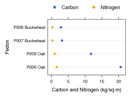
Total C and N Under Oak vs. Buckwheat
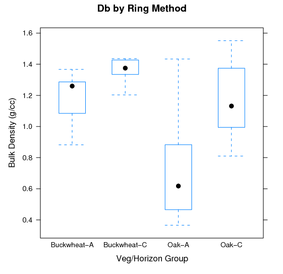
Islands of Fertility: Differences in Bulk Density: Variation in Db as a function of cover type and major horizon designation.
Analysis in R
### hypothesis : Db values for soils under oak will be less than those under buckwheat.
#### hypothesis: Db values for topsoil will be less than those for subsoil.

# read in the data
x <- read.csv('ring_samples_only.csv')

# make a new column with permutations of veg + horizon
x$veg_hz <- factor(with(x, paste(veg, '-', horizon, sep='')),
levels=c('b-a', 'b-c', 'o-a', 'o-c'),
labels=c('Buckwheat-A','Buckwheat-C','Oak-A','Oak-C'))

# some initial plots:

# all groups:
bwplot(db ~ veg_hz, data=x, ylab='Bulk Density (g/cc)', xlab='Veg/Horizon Group', main='Db by Ring Method')

# just veg
bwplot(db ~ veg, data=x, ylab='Bulk Density (g/cc)', xlab='Veg Group', main='Db by Ring Method')

# just horizon
bwplot(db ~ horizon, data=x, ylab='Bulk Density (g/cc)', xlab='Horizon Group', main='Db by Ring Method')


# some hypothesis tests:
# use lm for ANOVA, as design is not balanced

# full model: do any factors have an effect? interaction?
anova(lm(db ~ veg * horizon, data=x))
            Df  Sum Sq Mean Sq F value    Pr(>F)
veg          1 0.66902 0.66902  11.481 0.0021051 **
horizon      1 0.86462 0.86462  14.837 0.0006242 ***
veg:horizon  1 0.15915 0.15915   2.731 0.1095882
Residuals   28 1.63166 0.05827


#
# however, data is not normally dist, and sample size is small
#
# use non-parametric comparison:

# sig to 0.01 - 0.05
wilcox.test(db ~ veg, data=x, alternative='greater')
wilcox.test(db ~ veg, data=x, alternative='greater', subset=horizon == 'a')
wilcox.test(db ~ veg, data=x, alternative='greater', subset=horizon == 'c')


# one more approach:
par(mar=c(5,12,5,4), las=1)
plot(TukeyHSD(aov(db ~ veg_hz, data=x)))