
Simple Comparision of Two Least-Cost Path Approaches
Posted: Tuesday, February 19th, 2008
 Premise:
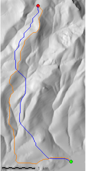
Simple comparison between the least-cost path as computed by r.walk vs. r.cost. Default parameters, unity travel friction, and λ = 1 were used with r.walk. Slope percent was used as the accumulated cost for r.cost. Test region similar to that used in a previous navigation example.
Results:
Code:
Prep work see attached files at bottom of page to re-create
# generate cost "friction" maps
# unity friction for r.walk
r.mapcalc "friction = 1.0"
# use slope percent as the friction for r.cost
r.slope.aspect elev=elev slope=slope format=percent
Compute the least-cost path via two methods
# compute cumulative cost surfaces
r.walk -k elev=elev friction=friction out=walk.cost start_points=start stop_points=end lambda=1
# Peak cost value: 14030.894105
r.cost -k in=slope out=cost start_points=start stop_points=end
# Peak cost value: 11557.934493

# compute shortest path from start to end points
r.drain in=walk.cost out=walk.drain vector_points=end
r.drain in=cost out=cost.drain vector_points=end
Vectorize least-cost paths for further analysis
r.to.vect -s in=walk.drain out=path_1
r.to.vect -s in=cost.drain out=path_2

# add DB column for length calculation
v.db.addcol path_1 columns="len double"
v.db.addcol path_2 columns="len double"

# how long are the two paths?
v.to.db path_1 option=length column=len units=me
# 6.03 km
v.to.db path_2 option=length column=len units=me
# 7.12 km
Simple map
d.rast shade
d.vect start icon=basic/circle fcol=green size=15
d.vect end icon=basic/circle fcol=red size=15
d.vect path_1 width=2 col=blue
d.vect path_2 width=2 col=orange
Sample the elevation raster at a regular interval
# add a vertex every 100m along each line
# this will create two tables for each
# path_1_pts_1   <-- original atts
# path_1_pts_2   <-- original cat + distance along the original line
v.to.points in=path_1 out=path_1_pts -i dmax=100
v.to.points in=path_2 out=path_2_pts -i dmax=100

# add column for elevation values
v.db.addcol map=path_1_pts layer=2 columns="elev double"
v.db.addcol map=path_2_pts layer=2 columns="elev double"

# upload elev values for profile graph
v.what.rast vector=path_1_pts raster=elev layer=2 column=elev
v.what.rast vector=path_2_pts raster=elev layer=2 column=elev

# dump profiles to CSV files
db.select path_1_pts_2 fs="," > p1.csv
db.select path_2_pts_2 fs="," > p2.csv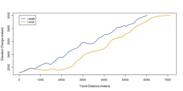
Least Cost Path Comparision Profile
Plot an elevation profile for each path
## startup R
R

## load data from previous steps
p1 <- read.csv('p1.csv')
p2 <- read.csv('p2.csv')

## can't guarantee that the two lines will be in the same direction (a r.to.vect thing?)
## p1 is correct, p2 is reversed

## make a nicer plot
## library(Cairo)
## Cairo(type='png', bg='white', width=800, height=400)

plot(elev ~ rev(along), data=p2, type='l', col='orange', lwd=2, xlab='Travel Distance (meters)', ylab='Elevation Change (meters)')
lines(elev ~ along, data=p1, col='RoyalBlue', lwd=2)
legend(0, 3000, legend=c('r.walk', 'r.cost'), col=c('RoyalBlue', 'orange'), lwd=2)
Attachments:
Links:
Mapping Wifi Networks with Kismet, GDAL, and GRASS
Raster Operations
Using R and r.mapcalc (GRASS) to Estimate Mean Topographic Curvature
