Home Projects Pedology and Soil Survey Other Information Pinnacles National Monument Soil Color Ideas

Soil Color Ideas

Premise

Soil color generally varies in a predictable pattern with depth according to surface vegetation, clay mineralogy and parent material. Highly contrasting parent geology influences soil color within Pinnacles via four main processes:

Original color of parent material
sedimentary sources: grey, yellow, white
granitic sources: yellow to orange
volcanic sources: pink, orange, white, green
Landscape age
older landscapes generally have redder hues (Fe-expression) from longer chemical weathering
Particle size distribution of parent material and the resulting field capacity of a soil formed from it
coarse textures result in lower field capacities, limiting vegetation growth and subsequent accumulation of organic matter in the surface horizons
Weathering rate of parent material
sedimentary materials derived from granitic sources (grey to yellow hues) have high levels of quartz and are therefore less susceptible to chemical weathering than volcanic rocks (redder hues)

Soil colors from Pinnacles: Moist colors in the L*U*V* color space (629 horizons).

Query Samples

All Horizons along with horizon thickness

SELECT x(pedon_spatial.wkb_geometry) AS x, y(pedon_spatial.wkb_geometry) AS y, horizon.pedon_id, (bottom - top) AS thick, m.r AS red, m.g AS green, m.b AS blue
FROM horizon JOIN munsell_lookup_v3 AS m
ON horizon.matrix_wet_color_hue = m.hue AND horizon.matrix_wet_color_value = m.value AND horizon.matrix_wet_color_chroma = m.chroma
JOIN pedon_spatial
ON pedon_spatial.pedon_id = horizon.pedon_id
WHERE matrix_wet_color_hue IS NOT NULL AND horizon.top != horizon.bottom
ORDER BY pedon_id ;

Horizon Thickness-weighted Average for Subsurface Horizons

SELECT x(pedon_spatial.wkb_geometry) AS x, y(pedon_spatial.wkb_geometry) AS y, a.pedon_id, a.red, a.green, a.blue FROM
        (
        SELECT horizon.pedon_id, sum(m.r * (bottom - top))/sum(bottom - top) AS red, sum(m.g * (bottom - top))/sum(bottom - top) AS green, sum(m.b * (bottom - top))/sum(bottom - top) AS blue
        FROM
        horizon JOIN munsell_lookup_v3 AS m
        ON horizon.matrix_wet_color_hue = m.hue AND horizon.matrix_wet_color_value = m.value AND horizon.matrix_wet_color_chroma = m.chroma
        WHERE matrix_wet_color_hue IS NOT NULL AND horizon.top != horizon.bottom AND horizon.bottom IS NOT NULL AND horizon.name !~*'O' AND horizon.top > 20
        GROUP BY pedon_id
        ) AS a
JOIN pedon_spatial
ON pedon_spatial.pedon_id = a.pedon_id ;

Pedon Color (spatially) Averaged within 500 meter grid, from profile thickness-weighted average

SELECT X(grid) AS x, Y(grid) AS y, avg(b.red) AS red, avg(b.green) AS green, avg(b.blue) AS blue, count(b.pedon_id) AS n_pedons
FROM
        (
        SELECT SnapToGrid(pedon_spatial.wkb_geometry, 500) AS grid, a.pedon_id, a.red, a.green, a.blue FROM
                        (
                        SELECT horizon.pedon_id, sum(m.r * (bottom - top))/sum(bottom - top) AS red, sum(m.g * (bottom - top))/sum(bottom - top) AS green, sum(m.b * (bottom - top))/sum(bottom - top) AS blue
                        FROM
                        horizon JOIN munsell_lookup_v3 AS m
                        ON horizon.matrix_wet_color_hue = m.hue AND horizon.matrix_wet_color_value = m.value AND horizon.matrix_wet_color_chroma = m.chroma
                        WHERE matrix_wet_color_hue IS NOT NULL AND horizon.top != horizon.bottom AND horizon.bottom IS NOT NULL AND horizon.name !~*'O' AND horizon.top > 20
                        GROUP BY pedon_id
                        ) AS a
        JOIN pedon_spatial
        ON pedon_spatial.pedon_id = a.pedon_id
        ) AS b
GROUP BY x,y ;

Visualization in R

Setup R environment

## load some libraries
library(sp)
library(spatstat)
library(plotrix)
library(Cairo)
library(Rdbi)
library(RdbiPgSQL)
 
## conn becomes an object which contains the DB connection:
conn <- dbConnect(PgSQL(), host="localhost", dbname="xxx", user="xxx", password="xxx")

Pinnacles Soil Color Map 1

Plot colors from all horizons, for all pedons. Note that a small amount of noise is added to the (x,y) coordinates of each pedon, so that the colors from each horizon do not overlap. Thinner horizons are depicted with a more transparent color.

## simple query
q1 <- "SELECT x(pedon_spatial.wkb_geometry) AS x, y(pedon_spatial.wkb_geometry) AS y, horizon.pedon_id, (bottom - top) as thick, m.r AS red, m.g AS green, m.b AS blue
FROM horizon JOIN munsell_lookup_v3 AS m
ON horizon.matrix_wet_color_hue = m.hue AND horizon.matrix_wet_color_value = m.value AND horizon.matrix_wet_color_chroma = m.chroma
JOIN pedon_spatial
ON pedon_spatial.pedon_id = horizon.pedon_id
WHERE matrix_wet_color_hue IS NOT NULL and horizon.top != horizon.bottom
ORDER BY pedon_id ;"
 
## run simple query
query <- dbSendQuery(conn, q1)
 
## fetch data according to query:
d <- dbGetResult(query)
 
## convert to spatial points data frame:
coordinates(d) <- c('x', 'y')
 
## rescale horizon thickness to the plotting symbol size range (1-3)
pch.size <- rescale(d$thick, c(0.5,3))
 
## simple plot
## plot(jitter(coordinates(d), 2), col=rgb(d$red,d$green,d$blue), pch=15, cex=pch.size)
 
 
## more interesting plot with the Cairo() output device
Cairo(type='png', file='pinn_colors.png', width=500, height=600)
 
plot(jitter(coordinates(d), 2), col=rgb(r=d$red, g=d$green, b=d$blue, alpha=0.75), pch=15, cex=pch.size, xlab='Easting', ylab='Northing', main='All Horizions')
 
dev.off()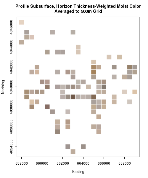

Pinnacles Soil Color Map 2

## more complex query computing profile weighted avg color, snapped to a grid
q2 <- "SELECT X(grid) AS x, Y(grid) AS y, avg(b.red) as red, avg(b.green) as green, avg(b.blue) as blue, count(b.pedon_id) as n_pedons
FROM
        (
        SELECT SnapToGrid(pedon_spatial.wkb_geometry, 500) AS grid, a.pedon_id, a.red, a.green, a.blue FROM
                        (
                        SELECT horizon.pedon_id, sum(m.r * (bottom - top))/sum(bottom - top) AS red, sum(m.g * (bottom - top))/sum(bottom - top) AS green, sum(m.b * (bottom - top))/sum(bottom - top) AS blue
                        FROM
                        horizon JOIN munsell_lookup_v3 AS m
                        ON horizon.matrix_wet_color_hue = m.hue AND horizon.matrix_wet_color_value = m.value AND horizon.matrix_wet_color_chroma = m.chroma
                        WHERE matrix_wet_color_hue IS NOT NULL AND horizon.top != horizon.bottom AND horizon.bottom IS NOT NULL AND horizon.name !~*'O' and horizon.top > 20
                        GROUP BY pedon_id
                        ) AS a
        JOIN pedon_spatial
        ON pedon_spatial.pedon_id = a.pedon_id
        ) AS b
group by x,y ;"
 
## run more complext query
query <- dbSendQuery(conn, q2)
 
## fetch data according to query:
d <- dbGetResult(query)
 
## convert to spatial points data frame
coordinates(d) <- c('x', 'y')
 
## set the transparency based on the number of pedons per 500m grid cell
a <- rescale(d$n_pedons, c(0.5,1))
 
## save plot to png with Cairo output device
Cairo(type='png', file='pinn_grid_colors.png', width=500, height=600)
plot(coordinates(d), col=rgb(r=d$red, g=d$green, b=d$blue, alpha=a), pch=15, cex=3, xlab='Easting', ylab='Northing', main='Profile Subsurface, Horizon Thickness-Weighted Moist Color\nAveraged to 500m Grid')
dev.off()

Colors of Pinnacles

library(colorspace)
 
## continuing from the first example query (all horizons)
 
## convert RGB triplets to RGB class object
d_cols <- RGB(d$red, d$green, d$blue)
 
 
## plot in RGB space:
Cairo(type='png', file='pinn_rgb.png', width=500, height=500)
par(pty='s')
plot(d_cols)
dev.off()
 
## plot in LUV space
Cairo(type='png', file='pinn_luv.png', width=500, height=500)
par(pty='s')
plot(as(d_cols, 'LUV'))
dev.off()

Can soil color be used to infer parent material source?
Approximate identification of parent material source based on soil colors. Note that this is a very coarse estimation, especially since large regions of the sedimentary materials were originally derived from granitic sources. The general trend visible in the clustering does match a rough approximation of the park geology.

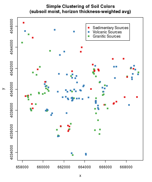
Pinnacles Soil Color Clustering Idea 1: PAM clustering of mean subsoil color (horizon thickness-weighted) for 170 pedons.

## load some libs
library(cluster)
library(RColorBrewer)
 
## cluster profile, depth-weighted average subsoi moist color
## note that there is a better clustering in the LUV color space
cols.pam <- pam( as(RGB(d$red, d$green, d$blue), 'LUV')@coords , k=3)
 
## open output device
Cairo(type='png', file='pinn_color_classes.png', width=500, height=600)
 
## make the map
plot(coordinates(d), col=brewer.pal(7, 'Set1')[cols.pam$clustering], cex=1, pch=15, main="Simple Clustering of Soil Colors\n(subsoil moist, horizon thickness-weighted avg)")
 
legend(664120, 4046262, legend=c('Sedimentary Sources', 'Volcanic Sources', 'Granitic Sources'), col=brewer.pal(3, 'Set1'), pch=15)
 
## done
dev.off()