
Terrain Classification Experiment 2: GRASS, R, and the raster package
Posted: Tuesday, May 24th, 2011
Quick post on terrain classification, based on some trouble folks were having with a previous example on Windows. With the spgrass6 package, raster stacks are created by loading several GRASS files at once: x <- readRAST6(vname=c('beam_sum_mj','ned10m_ccurv','ned10m_pcurv','ned10m_slope')). This works well on UNIX-like operating systems and in cases where the entire collection of raster maps can fit within the system memory. A different strategy is needed when working with massive raster stacks or on other (less useful) operating systems. This post outlines one possible strategy that should work on massive data sets, and across operating systems.
Outline
- export terrain surfaces from GRASS to intermediate files
- import into R with raster package
- perform unsupervised classification on a sample of the cells using PAM
- apply clustering to unsampled cells with randomForest
- save results to intermediate file
- import results into GRASS for post-processing
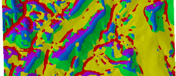
Image: Terrain Classification Example
This is by no means the best way of classifying terrain features, but it illustrates a work-flow that may be of interest to folks in the earth science community. Next up, a multi-scale approach to unsupervised landform classification.
Setup
# we previously used the spgrass6 package for raster I/O
# library(spgrass6)
library(cluster)
library(raster)
library(randomForest)

# setup region for terrain classification
system('v.to.rast --o in=FY2011 out=MASK use=val val=1')
system('g.region vect=FY2011 res=10 -ap')

# try loading raster data directly from GRASS database/location/mapset
# this does not use region / MASK information ...
# beam_sum <- raster('/home/dylan/grass/ca630/PERMANENT/cellhd/beam_sum_mj')

# need a different approach: export from grass to intermediate files
system('r.out.gdal --o -f type=Float32 in=beam_sum_mj out=/tmp/beam_sum.tif nodata=-9999')
system('r.out.gdal --o type=Float32 in=ned10m_ccurv out=/tmp/ned10m_ccurv.tif nodata=-9999')
system('r.out.gdal --o type=Float32 in=ned10m_pcurv out=/tmp/ned10m_pcurv.tif nodata=-9999')
system('r.out.gdal --o type=Float32 in=ned10m_slope out=/tmp/ned10m_slope.tif nodata=-9999')
Load intermediate files into R
# load temporary files that have identical grid topology
# (c/o the GRASS 'region' functionality)
beam_sum <- raster('/tmp/beam_sum.tif')
ccurv <- raster('/tmp/ned10m_ccurv.tif')
pcurv <- raster('/tmp/ned10m_pcurv.tif')
slope <- raster('/tmp/ned10m_slope.tif')

# re-class slope
m <- c(0,3,1,  3,15,2,  15,30,3, 30,45,4, 45,60,5, 60,Inf,6)
rclmat <- matrix(m, ncol=3, byrow=TRUE)
slope.rc <- reclass(slope, rclmat)

# stack
s <- stack(beam_sum, ccurv, pcurv, slope.rc)
layerNames(s) <- c('beam_sum', 'ccurv', 'pcurv', 'slope.rc')
Sample from original data, feed samples to PAM algorithm
# we can't operate on the entire set of cells,
# so we use one of the central concepts from statistics: sampling
# sample 10000 random points
s.r <- as.data.frame(sampleRegular(s, 10000))

# clara() function: need to remove NA from training set
s.r <- na.omit(s.r)
s.clara <- clara(s.r, stand=TRUE, k=5)
s.r$cluster <- factor(s.clara$clustering)
Use randomForest() to apply cluster rules at unsampled grid cells
rf <- randomForest(cluster ~ beam_sum + ccurv + pcurv + slope.rc, data=s.r, importance=TRUE, ntree=201)

# make predictions from rf model, along all cells of input stack
p <- predict(s, rf, type='response', progress='text')

# variable importance: all contribute about the same... good
importance(rf)
varImpPlot(rf)

# customized plot
par(mar=c(0,0,0,0))
plot(p, maxpixels=50000, axes=FALSE, legend=FALSE, col=brewer.pal('Set1', n=5))
Save predictions to an intermediate file
writeRaster(p, filename='/tmp/fy2011_5_class_geomorph.tif', overwrite=TRUE, datatype='INT1U', format='GTiff')GRASS: load terrain classes and finish processing
r.in.gdal --o in=/tmp/fy2011_5_class_geomorph.tif out=fy2011_5_class_geomorph
r.mapcalc "fy2011_5_class_geomorph.int = int(fy2011_5_class_geomorph)"
r.neighbors in=fy2011_5_class_geomorph.int out=fy2011_5_class_geomorph.int.5x5 size=5 method=mode
g.remove rast=fy2011_5_class_geomorph.int,fy2011_5_class_geomorph